In order to help exploration geoscientists better visualise key 3D seismic data within GIS, Exprodat recently experimented with importing seismic data into a voxel data cube for viewing in an ArcGIS Pro 3D scene.  

A voxel layer represents multidimensional spatial and temporal information in a 3D volumetric visualization. For example, think of a room. Imagine the room divided up into points, each, say, one metre apart. Every point will have a particular (x, y, z) coordinate. The coordinate is the distance from a particular corner of the room. At any given (x, y, z) point a data value (e.g. temperature) can be measured, so we have temperature as a function of (x, y, z). As we move around the room to other points, the temperature changes — increasing near the heat of spotlights and decreasing near a glass of cold beer.  

You can visualize atmospheric or oceanic data, a geological underground model, or space-time cubes as voxel layers. You can use voxel layers to explore spatial relationships with other content. For example, an underground model visualized as a voxel layer can be viewed together with boreholes or construction that is planned in an area.  

We thought a voxel layer would be an excellent container for 3D seismic amplitude information due to it also being volumetric, regularly gridded data.  

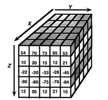
Figure 1: Schematic of a voxel cube – numbers representing the data value

ArcGIS Pro’s voxel functionality requires your data to be in NetCDF format and Pro provides tools to allow you to create these and load your data into them. Pro also provides tools to take advantage of voxel cube visualization and analysis capabilities.  

This blog describes how we implemented a repeatable workflow incorporating a custom Python toolbox to ingest 3D seismic data from Petrel into NetCDF format. 

1 – Exporting the seismic data from the interpretation project   

 Seismic data is essentially soundwaves shot into the ground with the response time recorded, and different seismic amplitudes are created depending on whether a rock layer is softer or harder than what is above it. A 3D seismic amplitude volume is like the room-temperature example in our introduction above except for two key differences: 

1. The vertical (z) axis is two-way travel time (TWT). 
2. The data values are seismic amplitudes, rather than temperature.  

We had a relatively small seismic cube measuring approximately 24 kms by 16 kms by 1.8 seconds. NetCDF format is a regular matrix of cubes meaning that each cube has the same dimension in X, Y, and Z directions. To ensure the output was a close representation of the seismic we decided to make timeslices that were vertically spaced close to the lateral spacing of 25m.  

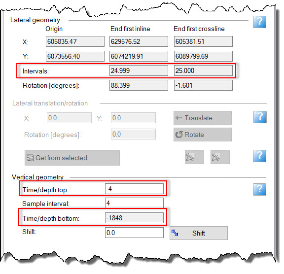
Figure 2: Seismic survey properties in Petrel

Performing an approximate time to depth calculation using a constant velocity value gave us a value for the cube’s thickness in metres, which allowed us to define the number of slices we needed to generate: 92.   

The next step was to extract the 92 time-slices from the interpretation package (Petrel). To do that we used a useful tool where you can extract the mean amplitude over a repeated time window. The settings for which are shown below. 

Figure 3: Repeated timeslice extraction in Petrel

Unfortunately, Petrel did not have an option to export straight to a .tif format raster so we exported those time–slices into a format which we could easily import into ArcGIS Pro using our Data Assistant add-in, e.g. ZMap+ grid format.  

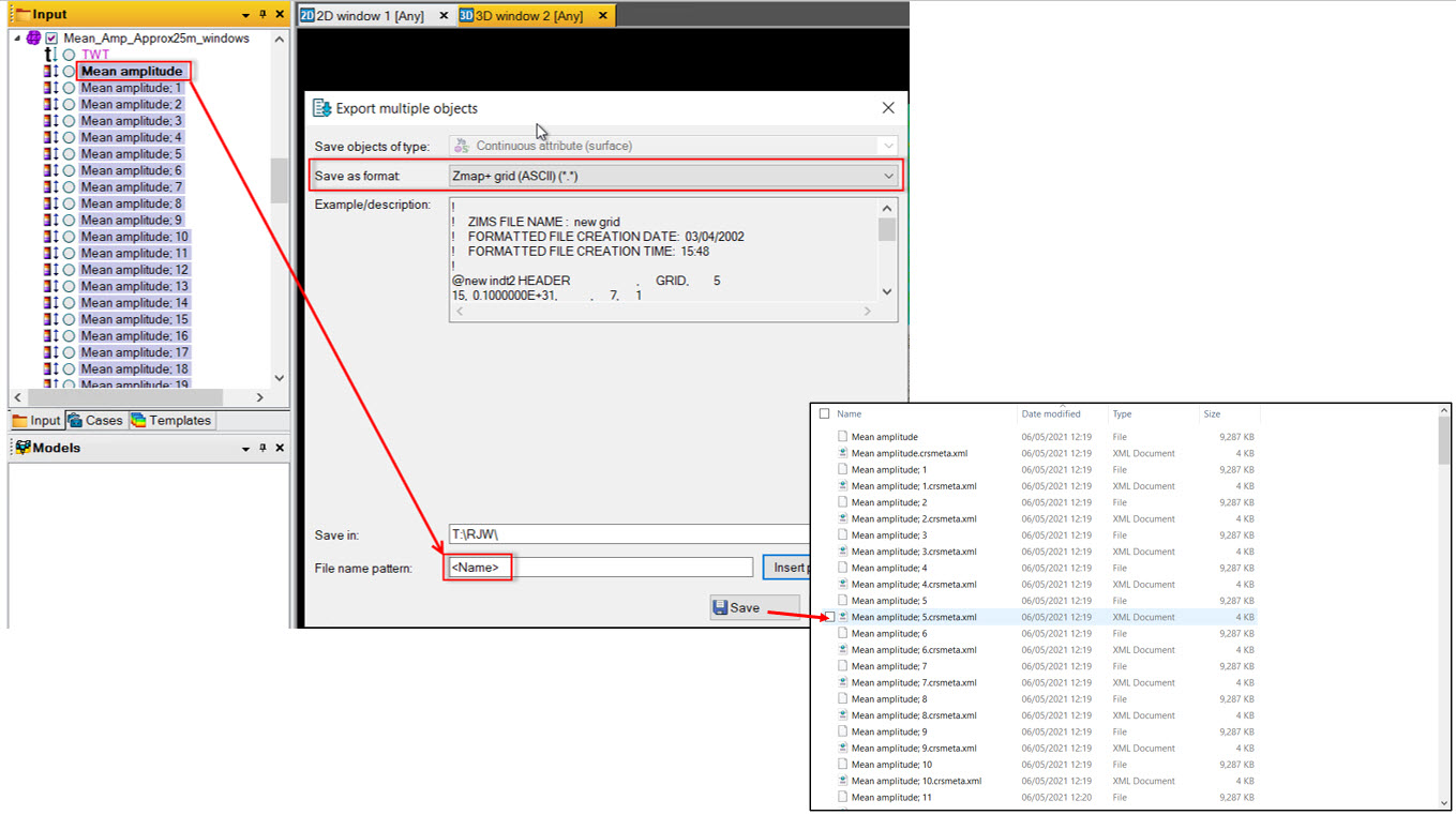
Figure 4: Exporting the timeslices from Petrel

2 – Converting seismic timeslices into useable grids 

We converted the time-slice grids into ArcGIS compatible rasters using Data Assistant, specifically its ‘Import All’ tool.  

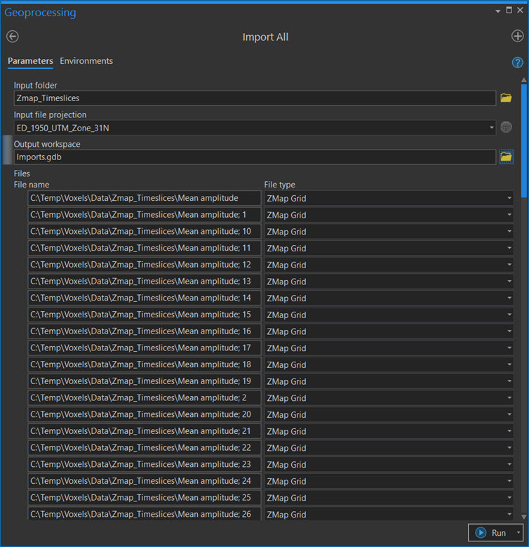
Figure 5: Importing all the timeslices using Data Assistant

We then used the ‘Copy Raster’ ArcGIS Pro geoprocessing tool in ‘Batch’ mode to convert these rasters into a .tif format ready to input into our Python toolbox. 

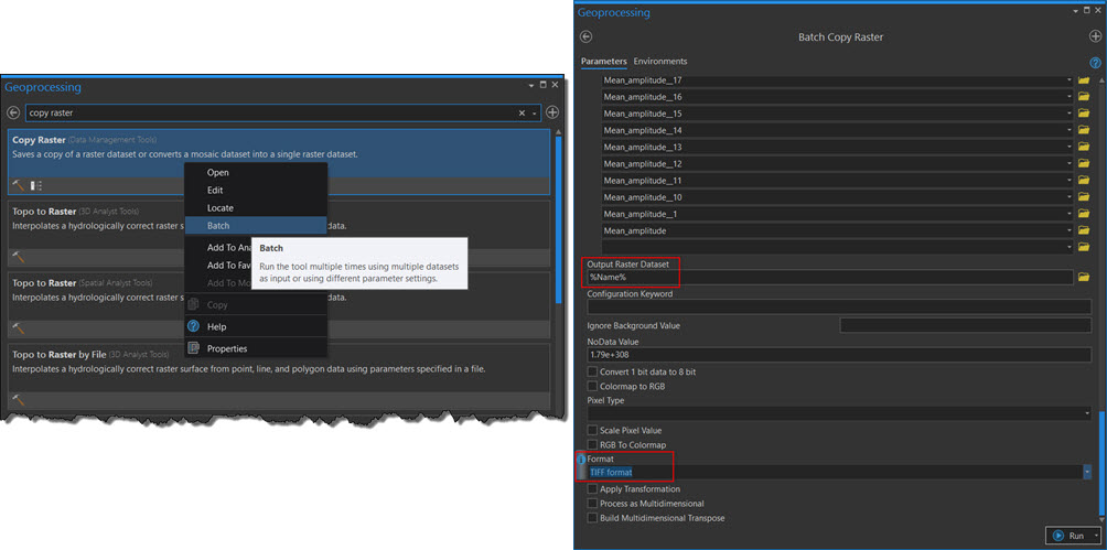
Figure 6: Batch running the Copy Raster geoprocessing tool

3 – Writing a Python toolbox 

Python toolboxes are ArcGIS geoprocessing toolboxes created entirely in Python. A Python toolbox and the tools contained within it look, act, and work just like regular ArcGIS toolboxes. 

Tools in a Python toolbox within ArcGIS provide many advantages, such as: 

• They behave just like a system geoprocessing tool—you can open them from the Catalog pane, use them in ModelBuilder, the Python window, and call them from another script. 
• You can write messages to the Geoprocessing history window and tool dialog box. 
• Using built-in documentation tools, you can provide documentation. 
• When a script is run as a script tool, arcpy is fully aware of the application it was called from. Settings made in the application, such as arcpy.env.overwriteOutput and arcpy.env.scratchWorkspace, are available from ArcPy in your script tool. 

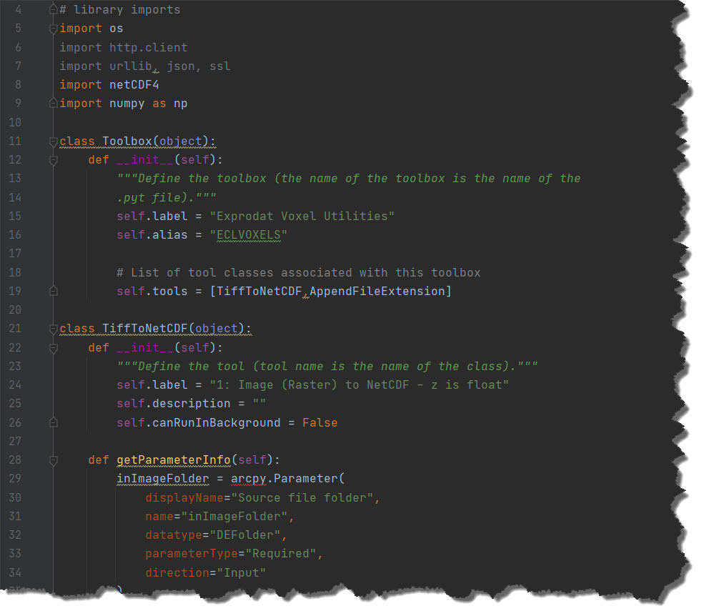
Figure 7: We used PyCharm to create and edit our toolbox

We created a Python toolbox tool that allows the following workflow to be executed and easily repeated: 

• Select the folder containing the rasters, and extract the seismic amplitude data from each raster. 
• Select file extension type to process (it will ignore other files in the folder if utilised). 
• The below set of depth parameters will place the voxel cube top at sea level and the bottom at -2305m below sea level (unit depends on the coordinate system of the map). 
• Output dataset is automatically designated as a NetCDF format with a .nc file extension.  
• User chooses the folder location and name.

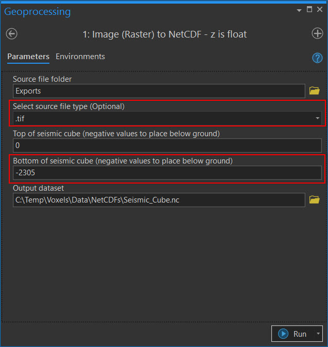
Figure 8: The toolbox tool ready to run

4 – The finished product 

We added the new NetCDF file to an ArcGIS Pro 3D Scene by navigating to the Map tab and clicking Add Data > Multidimensional Voxel Layer. We then selected the NetCDF as the Input Data Source and selected the seismic amplitude attribute ‘AMP’.

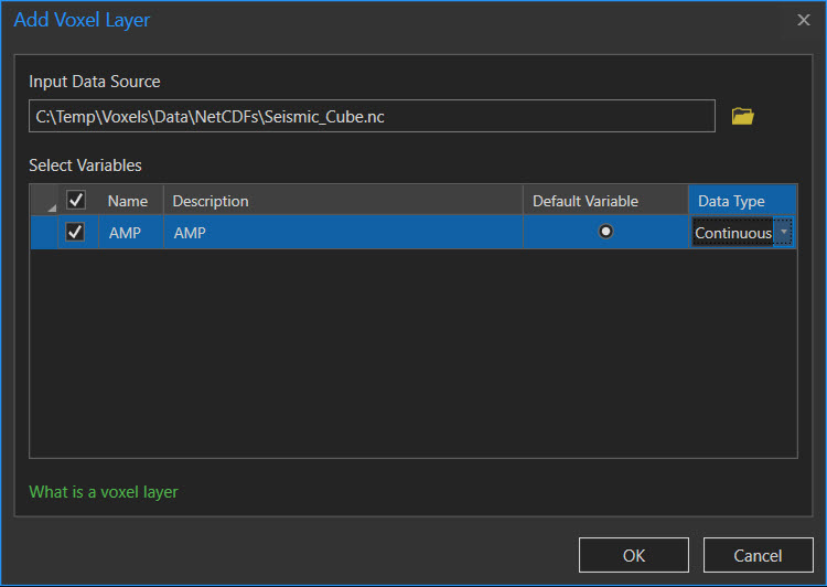
Figure 9: Adding the voxel layer to ArcGIS Pro

We imported the color bar from Petrel using Data Assistant’s handy ‘Convert Color Ramp’ tool, to ensure our Voxels cube looked just like the original seismic display in Petrel. 

Figure 10: Our voxel layer in a 3D Scene within ArcGIS Pro

We then investigated the built–in voxel visualisation functions including cutting across a particular fault of interest using the slice tool. Check out the video below of us cutting through the cube. 

The machine on which the video was rendered is a Dell XPS laptop with a 4GB nVidia GeForce GTX 1050 graphics card, an Intel I7-7700HQ CPU and 32Gb RAM.Finally, we explored the Data Filter and Transparency functions. In the screenshot below I have essentially cut out all the seismic amplitudes that do not represent a “very soft rock”. I would love to do that on a seismic cube with a calibrated sand presence amplitude (for those unfamiliar you can generate a seismic cube which has a particular amplitude range representing sandstone by calibrating the cube against wells). Just imagine the geobodies you could visualise! 

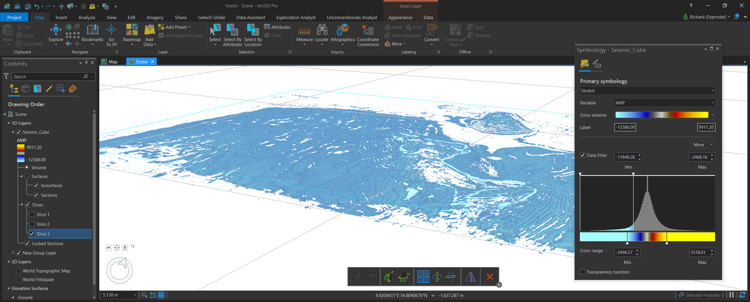
Figure 11: Data Filter option applied – showing only very soft responses

KeyFacts Energy Industry Directory: Exprodat